Detailed examples
This chapter will explain how the structure of the joint distribution model is created in virocon. The process of estimating the parameter values of a joint distribution, the “fitting” is explained in more detail by means of two examples. To create an environmental contour, first, we need to define a joint distribution. Then, we can choose a specific contour method and initiate the calculation. virocon uses so-called global hierarchical models to define the joint distribution and offers four common methods how an environmental contour can be defined based on a given joint distribution. Generally, virocon provides two ways of creating a joint model and calculating a contour. The first option is using an already predefined model, which was explained before in the quick start section (see Quick start example: Sea state contour). The second option is defining a custom statistical model, which is described in the following.
If the joint distribution is known, the procedure of calculating an environmental contour with virocon can be summarized as:
Load the environmental data that should be described by the joint model.
Define the structure of the joint model that we will use to describe the environmental data. To define a joint model, we define the univariate parametric distributions and the dependence structure. The dependence structure is defined using parametric dependence functions.
Estimate the parameter values of the joint model (fitting).
Define the contour’s return period and environmental state duration (for more detailed explanation see Environmental contour: useful definitions).
Choose a type of contour: IFormContour, ISormContour, DirectSamplingContour or HighestDensityContour (for more detailed explanation see Environmental contour: useful definitions).
50 year environmental contour: Hs-Tz DNVGL model
Here, we use a sea state dataset with the variables Hs (significant wave height) and Tz (zero-up-crossing period), fit the joint distribution recommended in DNVGL-RP-C203 1 to it and compute an IFORM contour. This example reproduces the results published in Haselsteiner et al. (2019) 2. Such a work flow is for example typical in ship design. The presented example can be downloaded from the examples section of the repository.
Imports
import numpy as np
import matplotlib.pyplot as plt

from virocon import (
read_ec_benchmark_dataset,
GlobalHierarchicalModel,
WeibullDistribution,
LogNormalDistribution,
DependenceFunction,
WidthOfIntervalSlicer,
IFORMContour,
plot_marginal_quantiles,
plot_dependence_functions,
plot_2D_contour,
)
Environmental data
This dataset has been used in a benchmarking exercise, see https://github.com/ec-benchmark-organizers/ec-benchmark . The dataset was derived from NDBC buoy 44007, see https://www.ndbc.noaa.gov/station_page.php?station=44007 . The datasets are available here: data.
data = read_ec_benchmark_dataset("datasets/ec-benchmark_dataset_A.txt")
Dependence structure
Define the structure of the joint model that we will use to describe the environmental data. To define a joint model, we define the univariate parametric distributions and the dependence structure. The dependence structure is defined using parametric functions. In this case, we used a 3-parameter power function and a 3-parameter exponential function as dependence functions. A dependence function must always contain a simple python function. Additionally we can constrain the functions parameters by supplying boundaries.
def _power3(x, a, b, c):
    return a + b * x ** c

def _exp3(x, a, b, c):
    return a + b * np.exp(c * x)
Parametric distributions
First, lower and upper interval boundaries for the three parameter values needs to be set. The dist_descriptions are
dictionaries that include the description of the distributions. The dictionary has the following keys depending on
whether the distribution is conditional or not: “distribution”, “intervals”, “conditional_on”, “parameters”. The key
“intervals” is only used when describing unconditional distributions while the keys “conditional_on” and “parameters”
are only used when describing conditional variables. The key “distributions” needs to be specified in both cases.
With “distribution” an object of distributions is committed. Here, we indicate the statistical
distribution which describes the environmental variable best. In “intervals” we indicate, which method should be used to
split the range of values of the first environmental variable into intervals. The conditional variable is then dependent
on intervals of the first environmental variable. The key “conditional_on” indicates the dependencies between the
variables of the model. Only one entry per distribution/dimension is possible. It contains either None or int. If the
first entry is None, the first distribution is unconditional. If the following entry is an int, the following
distribution depends on the first dimension as already described above. In “parameters” we indicate the dependency
functions that describe the dependency of the statistical parameters on the independent environmental variable.
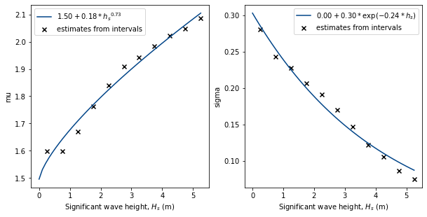
Here, dist_description_0 is the independent variable which is described by a Weibull distribution and split in equally sized intervals of width 0.5. dist_description_1 is described by a Lognormal distribution and is conditional on the first distribution (indicated by “conditional_on”: 0). The dependency of the individual parameters, mu and sigma of the Lognormal distribution are described by a power function and an exponential function.
bounds = [(0, None), (0, None), (None, None)]

power3 = DependenceFunction(_power3, bounds)
exp3 = DependenceFunction(_exp3, bounds)

dist_description_0 = {
    "distribution": WeibullDistribution(),
    "intervals": WidthOfIntervalSlicer(width=0.5),
}
dist_description_1 = {
    "distribution": LogNormalDistribution(),
    "conditional_on": 0,
    "parameters": {"mu": power3, "sigma": exp3}
}
Joint distribution model
In the following, the joint model is created from the dist description described above. Here, we are using global hierarchical models which are probabilistic models that covers the complete range of an environmental variable (’global’), following a particular hierarchical dependence structure. The factorization describes a hierarchy where a random variable with index i can only depend upon random variables with indices less than i 3 .
model = GlobalHierarchicalModel([dist_description_0, dist_description_1])
We define a semantics dictionary, that describes the model. This description can be used while plotting the contour.
semantics = {
"names": ["Significant wave height", "Zero-crossing period"],
"symbols": ["H_s", "T_z"],
"units": ["m", "s"],
}
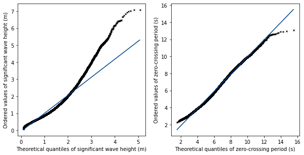
Fit the model to the data (estimate the model’s parameter values) and print the estimated parameter values. Afterwards, we create plots to inspect the model’s goodness-of-fit.
model.fit(data)
print(model)

fig1, axs = plt.subplots(1, 2, figsize=[10, 4.8])
plot_marginal_quantiles(model, data, semantics, axes=axs)
fig2, axs = plt.subplots(1, 2, figsize=[10, 4.8])
plot_dependence_functions(model, semantics, axes=axs)
The following plots are created:
Environmental contour
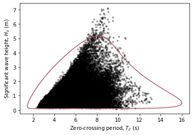
Compute an IFORM contour with a return period of 20 years and plot the contour on top of a scatter diagram of the metocean data.
state_duration = 1  # hours
return_period = 20  # years
alpha = state_duration / (return_period * 365.25 * 24)
contour = IFORMContour(model, alpha)

ax = plot_2D_contour(contour, sample=data, semantics=semantics, swap_axis=True)
plt.show()
- 1
DNV GL (2017). Recommended practice DNVGL-RP-C205: Environmental conditions and environmental loads.
- 2
Haselsteiner, A.F.; Coe, R.; Manuel, L.; Nguyen, P.T.T.; Martin, N.; Eckert-Gallup A. (2019): A benchmarking exercise on estimating extreme environmental conditions: methodology and baseline results. Proceedings of the 38th International Conference on Ocean, Offshore and Arctic Engineering OMAE2019, June 09-14, 2019, Glasgow, Scotland.
- 3
Haselsteiner, A.F.; Sander, A.; Ohlendorf, J.H.; Thoben, K.D. (2020): Global hierarchical models for wind and wave contours: physical interpretations of the dependence functions. OMAE 2020, Fort Lauderdale, USA. Proceedings of the 39th International Conference on Ocean, Offshore and Arctic Engineering.
50 year environmental contour: V-Hs-Tz
Warning
Stay tuned! We are currently working on this chapter. In the meantime if you have any questions feel free to open an issue.